Unsteady flow modeling is often fretted with instability issues. This is especially true when modeling mixed flow in an unsteady flow model due to the complexity of modeling a mixed flow regime (subcritical, supercritical, and hydraulic jumps). This complexity is associated with the nature of the unsteady flow equations (St. Venant equations). The St. Venant equation of Conservation of Momentum includes local acceleration and convective acceleration (inertial terms). When these unsteady flow calculations pass through critical depth, the algorithms become unstable because the derivatives become very large. These large derivatives cause oscillations in the solution, and the oscillations will grow larger until the model becomes unstable. In order to address this issue, Dr. Danny Fread (Fread, 1986) developed a methodology called the “Local Partial Inertia Technique.” This method has been adopted by HEC-RAS, and the following article will talk about the Mixed Flow option in HEC-RAS.
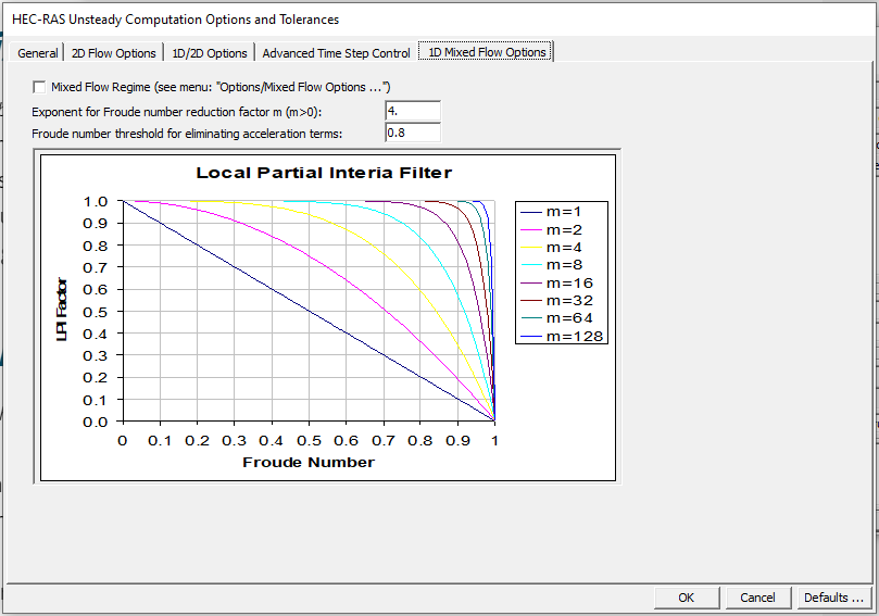
The Mixed Flow option in HEC-RAS unsteady flow modeling allows users to generate more stable models. This is because the Mixed Flow option dampens the effects of a significant amount of local acceleration. Specifically, when modelers use the Mixed Flow Regime setting, HEC-RAS will monitor the Froude number throughout the model simulation. When the Froude number starts to get close to one, the HEC-RAS will multiply the local acceleration term (also known as the Local Partial Inertia (LPI) Factor) by the numbers on the y-axis of the chart shown below. It is worth noting that there are some agencies that will not accept models that use the 1D Mixed Flow Options tab.
About the Local Partial Inertia (LPI) Method in HEC-RAS
In HEC-RAS, the Local Partial Inertia (LPI) method is applied using the LPI filter. Users can find this by navigating to the Unsteady Flow Analysis Window, clicking Options, navigating to Computation Options and Tolerances, and going to the 1D Mixed Flow Options tab.
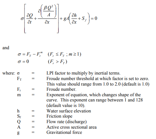
The LPI method applies a reduction factor to the two inertia terms (FT and m). By default, FT = 1.0 and m = 10. The modified momentum equation with these two factors is shown below. In other words, when the Froude number (Fr) is greater than 1.0, the LPI is set to zero. In HEC-RAS, the user can change the Froude number threshold and the exponent (m). As you increase the value of the Froude number threshold and exponent, model stability increases while accuracy decreases. In contrast, accuracy increases, and model stability decreases as you decrease the value of the Froude number threshold and exponent. The graph shown in the Mixed Flow Options in the Computation Options and Tolerances Dialog Box shows curves for the LPI factor at various exponents.
It should be noted that when the user turns on the mixed flow option by checking the box at the top of the 1D Mixed Flow Options tab, mixed flow is applied to the entire model (every reach, cross-section, and time step). However, there will be minimal effects when there are low Froude numbers, depending on how you set your LPI controls.