Manning’s roughness coefficient, which is also commonly referred to as Manning’s n, is an empirical parameter that represents energy loss due to a variety of things such as friction losses, flow separation, turbulence, and very sudden contractions or coefficients.
Relatively recently, the United States Army Corps of Engineers released versions of HEC-RAS that include two-dimensional (2D) hydraulic modeling features. As a result, 2D modeling is becoming more common, especially for certain types of projects such as dam breach inundation modeling, and floodplain mapping in densely populated urban areas.
One-dimensional (1D) and 2D HEC-RAS models have several things in common. For example, both 1D and 2D HEC-RAS models require the user to enter Manning’s roughness coefficients. However, “1D Manning’s n values” cannot be used interchangeably with “2D Manning’s n values.” The following article will describe how to add Manning’s n data to your HEC-RAS 2D model.
Manning’s for 2D Hydraulic Models
In a 1D hydraulic model, the applied Manning’s n values account for friction losses associated with surface roughness, drag losses associated with vegetation or channel obstructions, form losses due to turbulence, variations in geometry, bend losses in a channel, and other losses associated with uncertainty. However, in a 2D hydraulic model, some of the aforementioned losses are accounted for in the equations used to run the program. This is why “1D Manning’s n values” should not be used in a 2D hydraulic model.
There are many guidance documents and publications describing how to select an appropriate Manning’s n value for a 1D hydraulic model. Unfortunately, there are not nearly as many studies that provide guidance on selecting Manning’s n values for 2D models. However, it is generally accepted that Manning’s n values applied to 2D models are lower than those applied to 1D models.
An analysis performed by two engineers at Michael Baker International, Inc. involved developing a 1D model and a 2D model for four stream reaches without hydraulic structures. They then compared the results of the 1D and 2D models using identical Manning’s n values. The HEC-RAS 2D models generated higher water surface elevations. Next, the engineers performed an iterative analysis where they applied lower Manning’s n values until they generated water surface elevations equal to the 1D models. The following table showed the required decrease in Manning’s n value (as compared to the 1D model) required to achieve the same water surface elevation as the 1D models.
| Flow Path Complexity | Decrease in Manning’s n value (as compared to equivalent 1D model) |
|---|---|
| Simple Flow Path | 0% to 15% |
| Moderate Flow Path Complexity (Default) | 15% to 30% |
| Complex Flow Paths | 30% to 50% |
Manning’s n Values for 2D Hydraulic Models
Manning’s n-value recommendations for 2D hydraulic models are found in software documentation (e.g., the HEC-RAS 2D User’s Manual, the FLO-2D user’s manual, and the XPSWMM user’s manual).
The table below lists Manning’s n values that can be applied to 2D hydraulic modeling situations with non-shallow flow conditions.
| Land Use Type | Manning’s n Range |
| High-Density Residential Areas | 0.2 – 0.5 |
| Low-Density Residential Areas | 0.1 – 0.2 |
| Industrial/Commercial | 0.2 – 0.5 |
| Open Pervious Areas, minimal vegetation (grass) | 0.03 – 0.05 |
| Open Pervious Areas, moderate vegetation (shrubs) | 0.05 – 0.07 |
| Open Pervious Areas, thick vegetation (trees) | 0.07 – 0.12 |
| Waterways/channels – minimal vegetation | 0.02 – 0.04 |
| Concrete-Lined Channels | 0.015 – 0.02 |
| Paved Roads/Driveways | 0.02 – 0.03 |
| Lakes (no emergent vegetation) | 0.015 – 0.035 |
| Wetlands (emergent vegetation) | 0.05 – 0.08 |
| Estuaries/Oceans | 0.02 – 0.04 |
It is worth noting that Manning’s n values should be higher in areas with shallow flow depths and around buildings. Manning’s n values as high as 10 can be used to represent a building in a 2D hydraulic model. This high value accounts for the fact that buildings do not convey water.
How to Add Manning’s n Data to an HEC-RAS 2D Model
There are a couple of ways to add Manning’s n data to an HEC-RAS 2D model. The following sections of this article will describe some of the options available to HEC-RAS users.
Single Manning’s n value applied to entire the mesh area
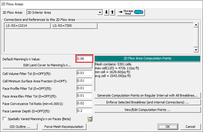
HEC-RAS users can apply a single Manning’s n value to an entire 2D mesh by navigating to the Geometric Data Editor and clicking the 2D Flow Area button located along the left side of the window. The default value is 0.06. The option to apply a single Manning’s n value to an entire 2D mesh is useful when initially setting up an HEC-RAS 2D model. It is always best to start simple and build complexity as you work out bugs and instabilities in the model.
Adding a Manning’s n layer
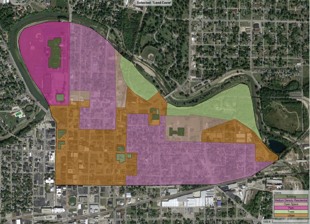
HEC-RAS allows the user to generate their own Manning’s n layer using geospatial data. The easiest way to develop a Manning’s n layer is to use a Geographic Information System (GIS) program such as ArcGIS or QGIS to draw land cover polygons on top of aerial imagery. An example is shown below.
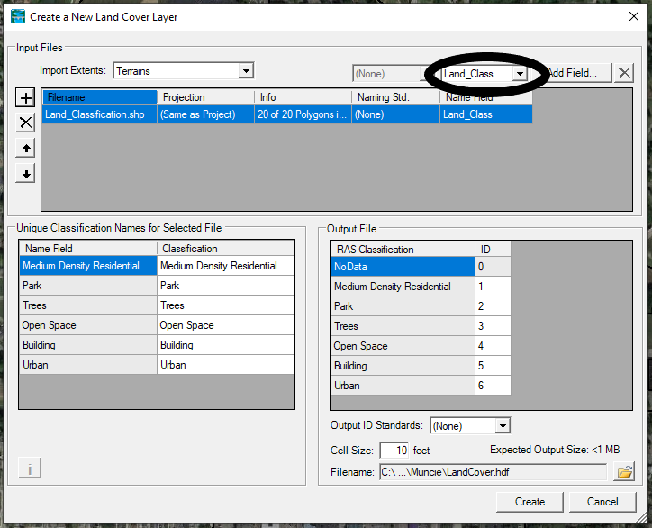
Then right-click Map Layers and select Create a New RAS Layer and Land Cover Layer. In the dialog box that pops up, click the “+” symbol on the left side and navigate to the land cover shapefile you created. Select the appropriate attribute field as shown below. Finally, click the Create button located in the lower right-hand corner.
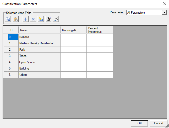
The created RAS Land Cover file will appear under Map Layers. Right-click the land cover file name and select Edit Land Cover Data Table. The window below will appear. Populate this table with the appropriate Manning’s n values and percent impervious values (optional).
Calibration Regions
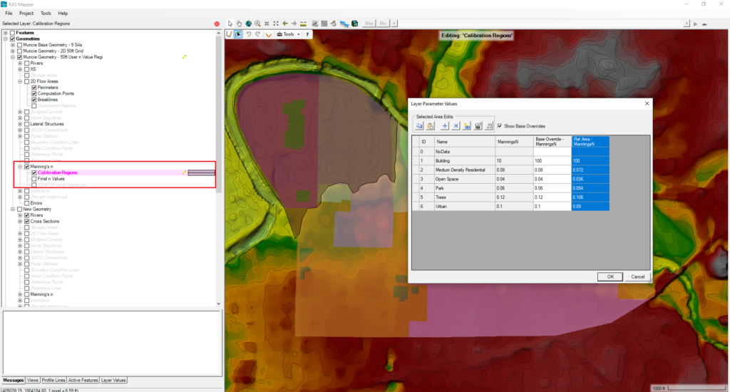
In HEC-RAS, Calibration Regions allow the user to refine a Manning’s n layer without having to go back and make a brand new land cover region. This is useful for calibration purposes because you can adjust Manning’s n values in areas where depths are a little too high or a little too shallow. You can only add a Calibration Region to an HEC-RAS plan that already has a Manning’s n layer associated with it.
Calibration Regions only apply to a specific Geometry and do not change the base land cover/Manning’s n-value layer. This means the user can apply different Calibration Regions to models that represent different flow conditions.
To add a Calibration Region to your HEC-RAS Model, go to RAS Mapper. In the contents panel, find the relevant geometry file. Then expand the Manning’s n menu under the geometry file’s name. Right-click Calibration Regions and select Edit Geometry. Draw a polygon to represent the desired Calibration Regions (see gray polygon in the image below). After you have drawn the polygon, right-click Calibration Regions and select Edit Manning’s n Values. Then populate the table with the new Manning’s n values.
More Information About Applying Manning’s n Values to HEC-RAS 2D Models
How does HEC-RAS apply Manning’s n values to a mesh?
Manning’s n values are applied to each cell face within a computational mesh. The Manning’s n value applied to a particular cell face is associated with the land cover/Manning’s n layer value at the center of the cell face. This is important to know because the modeler should create breaklines along areas where Manning’s n values change drastically.
Can you simulate vertical variation in Manning’s n with HEC-RAS 2D?
At this point, users cannot simulate vertical variation in Manning’s n values within HEC-RAS 2D. For this reason, it is important that modelers identify areas with shallow flows and increase Manning’s n values in those areas, which is particularly important when preparing a rain-on-grid model.